
# 主題式地圖
# Thematic map
# 開放式資料
# open data
# 地圖資料與社會經濟資料合併
# rgdal 套件
# tmap 套件
2022.7.28 更新R程式碼
# end
主題
本例說明考量社會經濟等開放式資料,輔以主題式繪圖方式,提升資料視覺化品質,便於資料呈現與溝通。下載資料的儲存目錄以C:\rdata為主。本範例包括以下六大步驟:
步驟1:下載社會經濟開放資料
步驟2:下載地圖資料
步驟3:匯入地圖資料至R
步驟4:匯入臺北市住宅竊盜點位資訊資料
步驟5:將臺北市住宅竊盜點位資訊整合至twn.taipei@data
步驟6:臺北市住宅竊盜分佈圖
下載網址:https://data.gov.tw/dataset/73886,參考圖-1,圖-2說明。

圖1-開放資料-臺北市住宅竊盜點位資訊


library(rgdal)
library(tmap)
# 匯入地理資料 readOGR {rgdal}
twn <- readOGR(dsn="C:/rdata/mapdata201805311056", layer="TOWN_MOI_1070516", encoding="UTF-8")
head(twn@data) # 中文亂碼
# 中文亂碼轉換 iconv {base}
twn@data$COUNTYNAME <- iconv(twn@data$COUNTYNAME, from = "UTF-8", to="UTF-8")
twn@data$TOWNNAME <- iconv(twn@data$TOWNNAME, from = "UTF-8", to="UTF-8")
head(twn@data) # 中文正常顯示
names(attributes(twn)) # 7個屬性
summary(twn) # 資料摘要
names(twn) # 7個欄位
class(twn) # SpatialPolygonsDataFrame
str(twn@data) # 368*7
# 篩選臺北市地理資料
twn.taipei <- twn[which(twn@data$COUNTYNAME == "臺北市"), ]
twn.taipei@data
str(twn.taipei@polygons[1])
str(twn.taipei@polygons[5])
# 將發生.現.日期由民國年轉為西元年
theft$發生.現.日期 <- as.Date(unlist(lapply(theft$發生.現.日期, function(x) {
if (nchar(x) == 6) return(paste0(as.numeric(substr(x,1,2))+1911, "-", substr(x,3,4), "-", substr(x,5,6)))
if (nchar(x) == 7) return(paste0(as.numeric(substr(x,1,3))+1911, "-", substr(x,4,5), "-", substr(x,6,7)))
})))
# 新增行政區欄位
# substr 函數與 Excel =MID函數 類似, 取出部分字串
theft$行政區 <- substr(theft$發生.現.地點,4,6)
# 篩選2018年&台北市資料
theft.2018 <- theft[theft$發生.現.日期 >= as.Date("2018-01-01") & substr(theft$發生.現.地點,1,3) == "台北市" ,] # 247*6
# 樞紐分析各行政區住宅竊盜次數小計
theaft.area <- aggregate(案類~行政區, data=theft.2018[c(2,6)], length)
names(theaft.area) <- c("行政區", "住宅竊盜發生數")
summary(theaft.area)
twn.taipei@data <- merge(twn.taipei@data, theaft.area, by.x = "TOWNNAME", by.y = "行政區", sort=FALSE)
twn.taipei@data
住宅竊盜發生數.color <- cut(twn.taipei@data$住宅竊盜發生數,
breaks=c(0,10,15,20,30,Inf),
labels=c("10以下", "11~15", "16~20", "21~30", "31以上"))
# 建立彩色調色盤(color palette)
# 內建調色盤 rainbow, heat.colors, terrain.colors, topo.colors, cm.colors, 本例以heat.colors為主
twn.taipei@data$Col <- heat.colors(5)[as.numeric(住宅竊盜發生數.color)]
plot(twn.taipei, col=twn.taipei@data$Col, main="2018年臺北市住宅竊盜分佈圖")
text(coordinates(twn.taipei)[,1], coordinates(twn.taipei)[,2], twn.taipei$TOWNNAME, cex=0.7)
legend("topright", legend=levels(住宅竊盜發生數.color), fill=twn.taipei@data$Col, col= heat.colors(5), title="住宅竊盜發生數")

# method 2 採用 qtm{tmap}
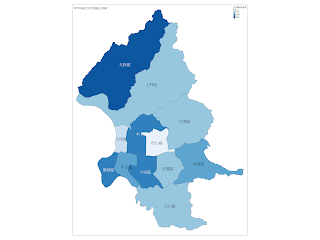
qtm(shp=twn.taipei, fill="住宅竊盜發生數", text="TOWNNAME", fill.title="住宅竊盜發生數", title="2018年臺北市住宅竊盜分佈圖")

qtm(shp=twn.taipei, fill="住宅竊盜發生數", text="TOWNNAME", fill.title="住宅竊盜發生數", title="2018年臺北市住宅竊盜分佈圖", fill.palette="Blues")
qtm(shp=twn.taipei, fill="住宅竊盜發生數", text="TOWNNAME", fill.title="住宅竊盜發生數", title="2018年臺北市住宅竊盜分佈圖", fill.palette="Greens")

步驟1:下載社會經濟開放資料
步驟2:下載地圖資料
步驟3:匯入地圖資料至R
步驟4:匯入臺北市住宅竊盜點位資訊資料
步驟5:將臺北市住宅竊盜點位資訊整合至twn.taipei@data
步驟6:臺北市住宅竊盜分佈圖
步驟1:下載社會經濟開放資料
本例以臺北市住宅竊盜點位資訊為例,資料筆數;1945,欄位個數:5,欄位名稱:編號,案類,發生(現)日期,發生時段,發生(現)地點。下載檔案:「臺北市10401-10709住宅竊盜點位資訊.csv」 。下載網址:https://data.gov.tw/dataset/73886,參考圖-1,圖-2說明。

圖1-開放資料-臺北市住宅竊盜點位資訊

圖2-臺北市住宅竊盜點位資訊CSV檔案
目前資料集已經下架, 請參考以下網址直接下載:
步驟2:下載地圖資料
參考政府資料開放平台,常用的地理資料包括下列二個項目:
1. 鄉鎮市區界線(TWD97經緯度),資料包括鄉(鎮、市、區)行政區域界線圖資。
下載網址:https://data.gov.tw/dataset/7441,參考圖-3說明。

圖3-鄉鎮市區界線下載
2. 直轄市、縣市界線(TWD97經緯度),資料包括直轄市以及縣(市)行政區域界線圖資
下載網址:https://data.gov.tw/dataset/7442,參考圖-4說明。

圖4-直轄市、縣市界線下載
本例考量分析台北市各區資料,因此下載第一項「 鄉鎮市區界線(TWD97經緯度)」,下載檔案為「 mapdata201805311056.zip」,解壓縮為「C:\rdata\mapdata201805311056」資料夾,參考圖-5說明。
地圖資料包括 .shp, .shx, .dbf, .prj,其中shp, shx, dbf 為三個必備檔案:
- .shp:圖形格式,用於儲存地圖元素的幾何資料。
- .shx:— 圖形索引格式,即幾何資料索引。記錄每一個幾何資料shp檔案之中的位置,能夠加快向前或向後搜尋幾何資料的效率。
- .dbf:屬性資料格式,以dBase IV的資料表格式儲存每個幾何形狀的屬性資料。
- .prj:圖形格式.shp檔案中幾何資料所使用的經緯度座標系統。

圖5-鄉鎮市區界線(TWD97經緯度)解壓資料夾
步驟3:匯入地圖資料至R
使用 rgdal 套件的 readOGR函數 以匯入地圖資料,使用 tmap 套件以製作主題式地圖
library(rgdal)
library(tmap)
# 匯入地理資料 readOGR {rgdal}
twn <- readOGR(dsn="C:/rdata/mapdata201805311056", layer="TOWN_MOI_1070516", encoding="UTF-8")
head(twn@data) # 中文亂碼
# 中文亂碼轉換 iconv {base}
twn@data$COUNTYNAME <- iconv(twn@data$COUNTYNAME, from = "UTF-8", to="UTF-8")
twn@data$TOWNNAME <- iconv(twn@data$TOWNNAME, from = "UTF-8", to="UTF-8")
head(twn@data) # 中文正常顯示
names(attributes(twn)) # 7個屬性
summary(twn) # 資料摘要
names(twn) # 7個欄位
class(twn) # SpatialPolygonsDataFrame
str(twn@data) # 368*7
# 篩選臺北市地理資料
twn.taipei <- twn[which(twn@data$COUNTYNAME == "臺北市"), ]
twn.taipei@data
str(twn.taipei@polygons[1])
str(twn.taipei@polygons[5])
步驟4:匯入臺北市住宅竊盜點位資訊資料
theft <- read.table("臺北市10401-10709住宅竊盜點位資訊.csv", header=TRUE, sep=",", stringsAsFactors=FALSE) # 2054*5# 將發生.現.日期由民國年轉為西元年
theft$發生.現.日期 <- as.Date(unlist(lapply(theft$發生.現.日期, function(x) {
if (nchar(x) == 6) return(paste0(as.numeric(substr(x,1,2))+1911, "-", substr(x,3,4), "-", substr(x,5,6)))
if (nchar(x) == 7) return(paste0(as.numeric(substr(x,1,3))+1911, "-", substr(x,4,5), "-", substr(x,6,7)))
})))
# 新增行政區欄位
# substr 函數與 Excel =MID函數 類似, 取出部分字串
theft$行政區 <- substr(theft$發生.現.地點,4,6)
# 篩選2018年&台北市資料
theft.2018 <- theft[theft$發生.現.日期 >= as.Date("2018-01-01") & substr(theft$發生.現.地點,1,3) == "台北市" ,] # 247*6
# 樞紐分析各行政區住宅竊盜次數小計
theaft.area <- aggregate(案類~行政區, data=theft.2018[c(2,6)], length)
names(theaft.area) <- c("行政區", "住宅竊盜發生數")
summary(theaft.area)
步驟5:將臺北市住宅竊盜點位資訊整合至twn.taipei@data
# merge函數中,sort參數須設定為FALSE,否則繪圖位置會有錯誤twn.taipei@data <- merge(twn.taipei@data, theaft.area, by.x = "TOWNNAME", by.y = "行政區", sort=FALSE)
twn.taipei@data
步驟6:臺北市住宅竊盜分佈圖
# method 1 採用 plot{graphics}住宅竊盜發生數.color <- cut(twn.taipei@data$住宅竊盜發生數,
breaks=c(0,10,15,20,30,Inf),
labels=c("10以下", "11~15", "16~20", "21~30", "31以上"))
# 建立彩色調色盤(color palette)
# 內建調色盤 rainbow, heat.colors, terrain.colors, topo.colors, cm.colors, 本例以heat.colors為主
twn.taipei@data$Col <- heat.colors(5)[as.numeric(住宅竊盜發生數.color)]
plot(twn.taipei, col=twn.taipei@data$Col, main="2018年臺北市住宅竊盜分佈圖")
text(coordinates(twn.taipei)[,1], coordinates(twn.taipei)[,2], twn.taipei$TOWNNAME, cex=0.7)
legend("topright", legend=levels(住宅竊盜發生數.color), fill=twn.taipei@data$Col, col= heat.colors(5), title="住宅竊盜發生數")

# method 2 採用 qtm{tmap}
qtm(shp=twn.taipei, fill="住宅竊盜發生數", text="TOWNNAME", fill.title="住宅竊盜發生數", title="2018年臺北市住宅竊盜分佈圖")

qtm(shp=twn.taipei, fill="住宅竊盜發生數", text="TOWNNAME", fill.title="住宅竊盜發生數", title="2018年臺北市住宅竊盜分佈圖", fill.palette="Blues")

qtm(shp=twn.taipei, fill="住宅竊盜發生數", text="TOWNNAME", fill.title="住宅竊盜發生數", title="2018年臺北市住宅竊盜分佈圖", fill.palette="Greens")

R程式碼 :
# title: 主題式地圖(Thematic map)-以政府開放資料為例
# date: 2018.10.28
# 本例說明考量社會經濟等開放式資料,輔以主題式繪圖方式,提升資料視覺化品質,使於資料呈現與溝通。

# 步驟1:
# 下載社會經濟等開放式資料,本例以臺北市住宅竊盜點位資訊為例,資料筆數;1945,欄位個數:5,欄位名稱:編號,案類,發生(現)日期,發生時段,發生(現)地點。
# 下載網址:https://data.gov.tw/dataset/73886

# 步驟2:下載地圖資料
# 本例考量分析台北市各區資料,因此下載第一項「 鄉鎮市區界線(TWD97經緯度)」,下載檔案為「 mapdata201805311056.zip」,解壓縮為「C:\rdata\mapdata201805311056」資料夾

# 下載世界地圖
# http://www.diva-gis.org/gdata


# 步驟3:匯入地圖資料至R
# 使用 rgdal 套件的 readOGR函數 以匯入地圖資料,使用 tmap 套件以製作主題式地圖

library(rgdal)
library(tmap)

# 匯入地理資料
twn <- readOGR(dsn="C:/rdata/mapdata201805311056", layer="TOWN_MOI_1070516", encoding="UTF-8")
head(twn@data) # 中文亂碼

# twn <- readOGR(dsn="C:/rdata/TWN_adm", layer="TWN_adm1", encoding="UTF-8")
head(twn@data) # 中文亂碼
names(twn@data)

# 中文亂碼轉換 iconv
twn@data$COUNTYNAME <- iconv(twn@data$COUNTYNAME, from = "UTF-8", to="UTF-8")
twn@data$TOWNNAME <- iconv(twn@data$TOWNNAME, from = "UTF-8", to="UTF-8")
head(twn@data) # 中文正常顯示

names(attributes(twn)) # 7個屬性
summary(twn) # 資料摘要
names(twn) # 7個欄位
class(twn) # SpatialPolygonsDataFrame
str(twn@data) # 368*7

# 篩選臺北市地理資料
twn.taipei <- twn[which(twn@data$COUNTYNAME == "臺北市"), ]
twn.taipei@data

str(twn.taipei@polygons[1])
str(twn.taipei@polygons[5])

# 步驟4:匯入臺北市住宅竊盜點位資訊資料
theft <- read.table("臺北市10401-10709住宅竊盜點位資訊.csv", header=TRUE, sep=",", stringsAsFactors=FALSE) # 2054*5

# 將發生.現.日期由民國年轉為西元年
theft$發生.現.日期 <- as.Date(unlist(lapply(theft$發生.現.日期, function(x) {
 if (nchar(x) == 6) return(paste0(as.numeric(substr(x,1,2))+1911, "-", substr(x,3,4), "-", substr(x,5,6)))
 if (nchar(x) == 7) return(paste0(as.numeric(substr(x,1,3))+1911, "-", substr(x,4,5), "-", substr(x,6,7)))
})))

# 新增行政區欄位
theft$行政區 <- substr(theft$發生.現.地點,4,6)

# 篩選2018年&台北市資料
theft.2018 <- theft[theft$發生.現.日期 >= as.Date("2018-01-01") & substr(theft$發生.現.地點,1,3) == "台北市" ,] # 247*6

# 樞紐分析各行政區住宅竊盜次數小計
theaft.area <- aggregate(案類~行政區, data=theft.2018[c(2,6)], length)
names(theaft.area) <- c("行政區", "住宅竊盜發生數")
summary(theaft.area)

# 步驟5:將臺北市住宅竊盜點位資訊資料整合至 twn.taipei@data
# merge函數中,sort參數須設定為FALSE,否則繪圖位置會有錯誤
twn.taipei@data <- merge(twn.taipei@data, theaft.area, by.x = "TOWNNAME", by.y = "行政區", sort=FALSE)
twn.taipei@data

# 步驟6:臺北市住宅竊盜分佈圖

# method 1 採用 plot{graphics}
住宅竊盜發生數.color <- cut(twn.taipei@data$住宅竊盜發生數,
 breaks=c(0,10,15,20,30,Inf),
 labels=c("10以下", "11~15", "16~20", "21~30", "31以上"))

# 建立彩色調色盤(color palette)
# 內建調色盤 rainbow, heat.colors, terrain.colors, topo.colors, cm.colors, 本例以heat.colors為主
twn.taipei@data$Col <- heat.colors(5)[as.numeric(住宅竊盜發生數.color)]

plot(twn.taipei, col=twn.taipei@data$Col, main="2018年臺北市住宅竊盜分佈圖")
text(coordinates(twn.taipei)[,1], coordinates(twn.taipei)[,2], twn.taipei$TOWNNAME, cex=0.7)
legend("topright", legend=levels(住宅竊盜發生數.color), fill=twn.taipei@data$Col, col= heat.colors(5), title="住宅竊盜發生數")

# method 2 採用 qtm{tmap}
qtm(shp=twn.taipei, fill="住宅竊盜發生數", text="TOWNNAME", fill.title="住宅竊盜發生數", title="2018年臺北市住宅竊盜分佈圖")

qtm(shp=twn.taipei, fill="住宅竊盜發生數", text="TOWNNAME", fill.title="住宅竊盜發生數", title="2018年臺北市住宅竊盜分佈圖", fill.palette="Blues")

qtm(shp=twn.taipei, fill="住宅竊盜發生數", text="TOWNNAME", fill.title="住宅竊盜發生數", title="2018年臺北市住宅竊盜分佈圖", fill.palette="Greens")
# end